Process Mining from Unstructured Text

Why?

Current SOTA approaches to autonomous systems (like the agents used in Rival’s platform) reason and act in unstructured text using frameworks such as CoT and ReAct. While powerful and flexible, this presents huge challenges in understanding what an agent does at scale without manual consumption of unstructured logs and “agent trajectories”.

This understanding is necessary to implement capabilities required of these systems to solve real problems and operate at high-stakes enterprise scale, such as:

• Reactive failure analysis
• Statistically informed system improvements
• Proactive real-time control and monitoring

The focus of Traditional ways to perform analysis of complex processes are techniques which usually require highly structured, discrete event logs - not blobs of unstructured text. The goal of our project Taxi (see the blogpost!) is to extract usable insights from complex agentic processes, so we'll have to bridge this gap.

The Pipeline

Practitioners can transform large amounts of agent reasoning into discrete steps by taking advantage of the same semantic embeddings that power modern vector-RAG.

Traditional vector RAG starts by extracting a vector for each item in a collection of texts that represents the “meaning” of the text. These can be used to recover texts relevant to a search term by calculating a vector for the term, calculating the mathematical similarity between each text vector and the search vector, and returning the most similar items.

Semantic clustering works similarly, but uses traditional ML algorithms to group (cluster) texts based on their similarity to each other instead of a search term. These clusters are taken to represent abstract topics or steps during further analysis, and an LLM can be used to assign names to each cluster based on its members, hopefully providing interpretable titles to the discovered abstract concepts.

For example, in conversation logs, there might be hundreds of nuanced ways one speaker greets another. This technique might discover that “Hello”, “Hi”, “What’s Up”, (and so on) are all close to each other when represented as vectors, and belong to the same discrete cluster. After this grouping, a smart LLM understands that all the members of this cluster are forms of greetings, and assigns a generic name “Greeting” to the group.

These abstract labeled clusters can be used downstream for any number of critical tasks - such as understanding which kinds of step flows are correlated with failure or success, or even generating a flowchart that represents the decision-making made by the agent across thousands of executions.

Challenge - How to Choose a Pipeline?

This seems extremely powerful - and it is! At Rival, we even used similar approaches in recent benchmarking work to understand and improve our own agents.

But there are three critical decisions when designing such a pipeline, each with potential huge ramifications in performance:

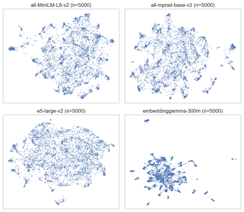
• Embedding Model: Not all models are the same, and different embedding vectors emphasize different aspects of text. As an example, here is a UMAP plot of the same 5000 sentences from our experiment in embedding space under different models:

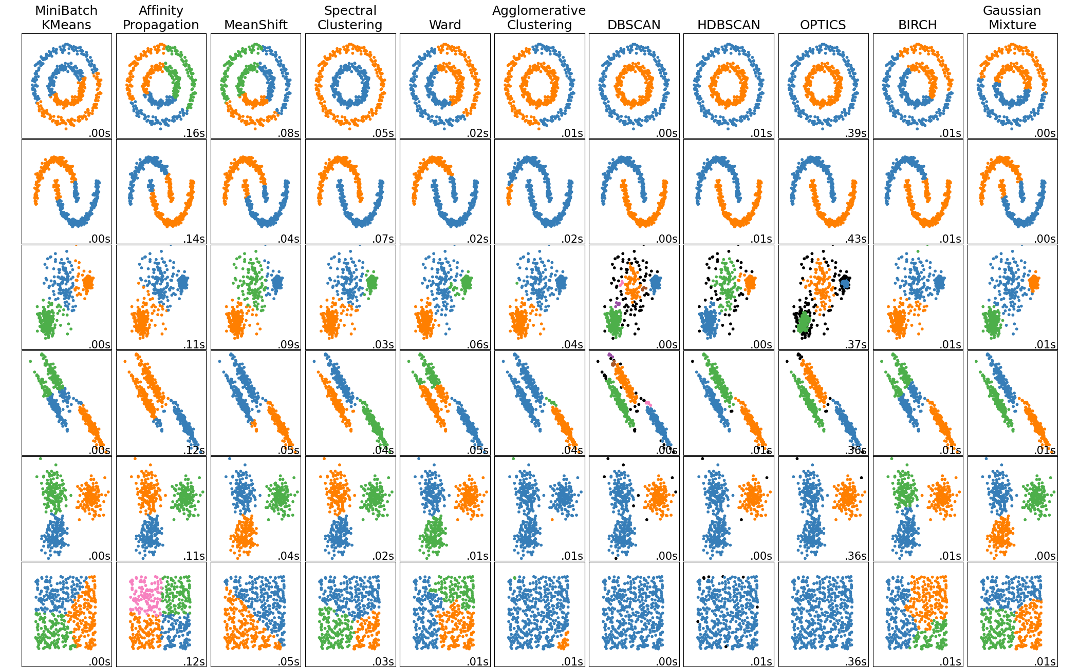
• Clustering Algorithm: Different clustering algorithms make decisions based on different aspects of the data and make assumptions about what a cluster should look like. A common image used to emphasize this point from scikit-learn’s documentation:

• LLM Labeling Technique: While irrelevant to cluster discovery the information provided to the LLM has an impact on the quality of the name it decides on for the end cluster.

Making a Decision

So how do you choose? When we initially wanted to use this technique, we assumed that there would be robust experimental work we could draw on to ensure we were choosing the best approach. We were shocked to find that existing work was far from helpful.

The standard MTEB benchmark used to assess embedding cluster performance operates against a fixed set of ground truth labels, penalizing clusters that are potentially correct but overly specific. Example: the difference between a single cluster “Greeting” and two clusters {“Formal Greeting”, “Informal Greeting”} might be a good thing.

The benchmark also does not test the quality of the assigned name itself - it is just used to check whether the labeled cluster structure is able to be reconstructed by embedding clusters.

In order to do this properly, we realized we would have to test this ourselves.

The Experiment - ClosedCaption

Experimental Data

This experiment is based on natural language data from the Massive Text Embedding Benchmark (MTEB). The full benchmark dataset is intended to test the broad performance of text embeddings, and contains 58 datasets over 112 languages that test quality over 8 different tasks that embeddings are commonly used for (only one of which is clustering).

The MTEB datasets for clustering are split into longer paragraphs and shorter sentences. For this experiment, we used the RedditClustering dataset, which contains the title of thousands of Reddit posts for 50 different subreddits, with the originating subreddit considered the “ground truth”.

Measurement of Topic Quality

Issues with “Out-of-the -Box” MTEB

The standard MTEB assessment of embedding clustering quality is a run of MiniBatchKMeans with K set equal to the known ground truth number of clusters.

The “V-Measure” of the resulting clusters is then taken with respect to the ground truth - a harmonic average score of the Homogeneity (do clusters contain only data points from a single class?) and Completeness (are all data points of a single class assigned to the same cluster?) scores.

This approach does not directly answer the “end-to-end” aspect of our use-case: how to build an embedding-cluster-label pipeline that yields the highest quality assignment to natural language topics.

But we were hesitant to even rely on MTEB leaderboard to analyze the embedding-to-cluster component due to two important shortcomings:

1. The ground truth labels penalize systems that find potentially valid groupings not aligned with the ground truth (either more specific, or assignment using a different set of parameters)
2. Using K-Means with a known value for K does not demonstrate embedding performance on successfully mining topics without prior knowledge of how many topics exist, which is a key interest in our use-case.

To overcome these challenges and actually answer our question, we need both a different approach and a better metric.

Our Approach: Clustering Scores as Binary Classification

The key intuition behind the metrics we used for analysis is that the quality of a cluster can be defined based on how “easy” it is to differentiate between items inside and outside of the cluster.

In other words - once individual items are assigned to cluster labels, the quality of an individual cluster can be tested based on how well an “expert” system WITHOUT prior knowledge of tjhe clustering assignments is able to reconstruct which items belong (and do not belong) to a cluster given only the label.

This treats the quality of a cluster category as a binary classification task from the perspective of the expert system, with the confusion matrix below.

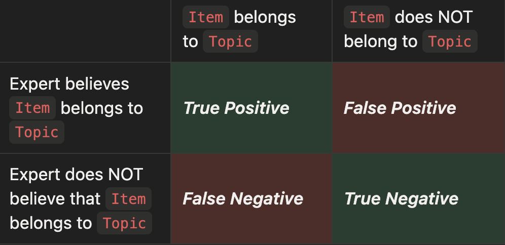
Traditional metrics for binary classification, such as precision, recall, F1, etc. can then be used as scores for individual clusters, and a weighted score based on the size of each cluster can be used to determine overall quality. Important to note is potential bias to fewer clusters - when the system generates fewer groups, it is harder to mis-assign items.

As is in vogue, our “Expert System” is an LLM-as-a-judge based on Gemini 2.5 Pro. The LLM was provided with a category name and a mixed set of items from and outside the category, and instructed to determine which of the items in the set truly belonged to the category, and which were impostors.

‍

Experimental Parameters

Embedding Models

Our experiment tested the following embedding models from HuggingFace in the SentenceTransformers library:

1. all-MiniLM-L6-v2
   
   • Specs: 384 dimensions, 22M parameters, released August 2021
   • ‍Architecture: 6-layer bidirectional Transformer distilled from larger BERT models
2. embeddinggemma-300m
   
   • Specs: 768 dimensions, ~300M parameters, released September 2025
   • ‍Architecture: Adapted from Gemma LLM into a bidirectional encoder
   • ‍Key Features: Instruction-tuned (supports task-specific prefixes to alter embedding space based on goal), supports Matryoshka Representation Learning (allows vectors to be truncated while maintaining high performance)
3. all-mpnet-base-v2
   
   • Specs: 768 dimensions, 110M parameters, released August 2021
   • ‍Architecture: Bidirectional Transformer trained with Masked and Permuted Pre-training
4. e5-large-v2
   
   • Specs: 1024 dimensions, 335M parameters, released December 2022
   • ‍Architecture: 24 layer bidirectional transformer, based on BERT-large
   • ‍Key Features: Instruction-tuned (requires specific prefixes for clustering or document retrieval)

LLM-Labeling Techniques

• Flat Labeling: Instructed to label a cluster just based on text samples from within the cluster and text sampled from outside the cluster.
  • Sampling from outside the cluster is weighted by its closeness to the cluster to ensure that we don’t provide easy negative examples
• Agent Labeling: Similar to the flat labeling, but the LLM is also given a semantic search tool that enables it to explore the most similar in-cluster and out-of-cluster texts to a search term.
• Tree Labeling: Most of the clustering methods (except standard KMeans and flat Leiden) create a full hierarchy of clusters (see the image):
  • A root cluster contains all of the items
  • Child clusters recursively contain a partition of the items in the parent.
  • For these, the LLM started at the root and was recursively instructed to label each of the children at once based on the nuances that differentiated between them.

‍

Clustering Algorithms

We focused on algorithms that scale reasonably well to larger datasets, incorporating those that cluster based on embedding distance, density, and graph structure.

• Minibatch-KMeans: Instead of manually specifying a value for K, we performed a sweep across values of k from 10 to 100 and choose the result with the best silhouette score.
• HDBSCAN on top of a 50-K-Nearest-Neighbors Graph
• Leiden Community Discovery on top of a 50-K-Nearest-Neighbors graph, using three different approaches:
  • A single traditional pass with the standard resolution of 1.0
  • An iterative resolution refinement that constructs a tree of clusters
  • Recursive splitting with a constant resolution of 0.5 to build a tree of clusters
• Bisecting-KMeans (k=2) to build a binary tree hierarchy of clusters

Results

TL;DR Conclusions

1. We found that the most critical factors in end-result quality were, in descending order:
   1. Selection of the clustering algorithm
   2. Architecture of the LLM naming system
   3. Selection of the embedding model
2. While imperfect, distance in embedding space can be seen as a proxy for lower bound on concept similarity (as opposed to the common treatment of such distance as expected similarity) - with potentially different

Overall Performance

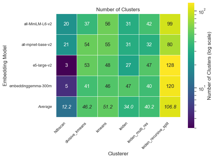
Unsurprisingly, we found that the biggest differentiator in overall performance (as measured by the Matthews Correlation Coefficient) is the clustering algorithm used - note the higher variance across the rows versus the columns:

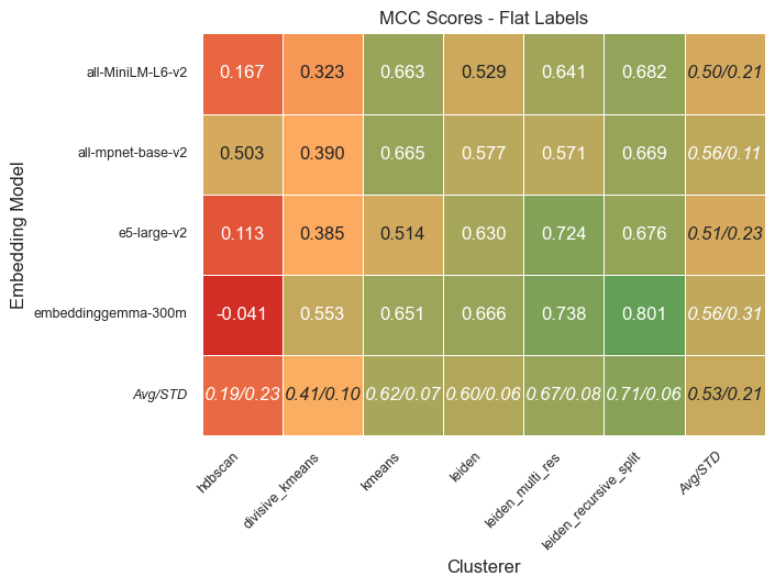
Adjusting hyperparameter values would cause each of these algorithms to behave differently, however, our initial hyperparameter values across different configurations resulted in a relatively consistent number of clusters across most algorithms:

Clusterer Differences

In order to fully understand the performance of these algorithms, it is useful to consider the properties of both the lowest (HDBSCAN) and the highest (Leiden-based) performing clusterers in relation to embedding space.

HDBSCAN detects clusters by looking for regions of high density. This is an approach which can collapse in high-dimensional embedding space, where the “curse of dimensionality” causes the contrast between dense and sparse regions vanishes as datapoints become roughly equidistant.

To see this effect visually, examine the distribution of distances between high-dimensional embeddings versus the same embeddings scaled down - in the original “raw” space, most embeddings have the same distance from each other in a sharp peak, while in the dimensionally reduced space, the distances have much more nuance.

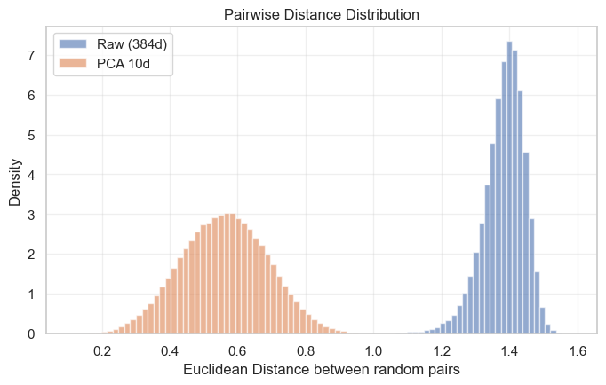
Most existing use of HDBSCAN on embedding vectors negates this by applying dimensionality reduction as a necessary preprocessing step. We did not, as it would have introduced another hyperparameter that needed to be tuned, and our goal was to study the robustness of these techniques.

Unlike density-based methods, Leiden treats clustering as a community detection problem rather than a geometric one. By first constructing a K-Nearest-Neighbors (KNN) graph, Leiden  decouples the clustering logic from the raw metric space - agnostic to the specific geometry of the high-dimensional embeddings. By focusing instead on topological connectivity (who is connected to whom), Leiden bypasses the noise of the embedding space and successfully recovered granular, semantically coherent structures

LLM-as-a-Judge MCC versus Silhouette Score

Silhouette Score is one of the most common methods to measure the quality of an individual cluster, and is calculated by measuring how similar clusters are to themselves versus other clusters. Conveniently enough, the score has the same range as MCC, from -1 (crap cluster) to +1 (good cluster)!

Examining the correlation between the LLM judge’s MCC score and the silhouette score of each individual labeled cluster across all of our tests, we note an interesting effect:

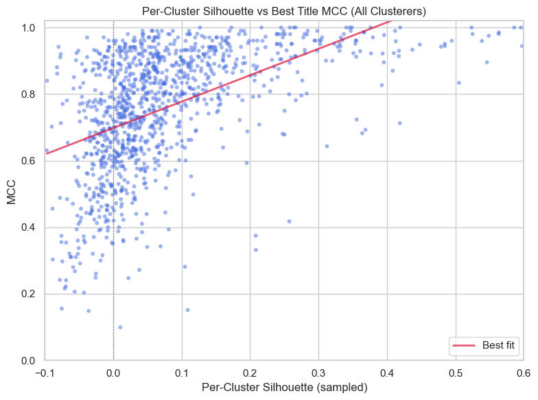
A cluster’s silhouette score offers a decent “lower bound” on the quality of an LLM-assigned label. Clusters with a high silhouette score are “easy” to name, with proportionally better LLM labels. However, a low silhouette score does not necessarily mean a poorly named cluster.

The critical takeaway: embedding geometry is a good, but flawed proxy for semantic interpretability, and we need algorithms (like Leiden) that don't depend on that geometry being perfect.

Performance Gain of Labeling Strategies

Across all embedding types and clustering algorithms, both agentic and tree-based labeling strategies lead to statistically significant gains in performance across precision and specificity metrics, at the price of a smaller decrease in Recall.

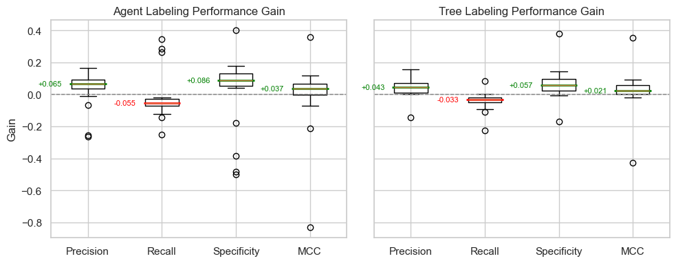
This change is not surprising, as both the Agentic and Tree generation approach push the LLM towards more specific labels that are easier to discriminate, but may accidentally lead to excluding items that should be included.

To see this effect, let’s examine individual clusters that have a large increase in MCC when named by an agent instead of the “flat” labeling across all of our experiments:

It is worth noting that the agentic approach seems especially suited for naming clusters where the distinguishing feature is a kind of meta-feature - such as the two above examples where the cluster was correctly defined by the language, not the subject itself.

Final Thoughts on Shortcomings

The text-embedding-LLM label pipeline is incredibly helpful to discover interpretable categories in natural language data, and is especially useful when coupled with downstream analysis and visualization.

However, we have found two key shortcomings of this approach.

Arbitrariness of Embedding Space

Off-the-shelf semantic embeddings restrict discovery to categories that the embedding space already considers to be close. This does not easily allow for specifying attributes that may be more relevant for the downstream analysis.

One potential way to solve this issue is the use of “instruction-tuned” semantic embeddings, which can have natural language task instructions affect the features of the calculated embedding.

Misalignment with Process Mining

If the individual pieces of text come from a larger process (such as our use-case at Rival for reasoning trajectories), embedding them in isolation destroys the information given by their position in the process as a whole.

By using these embeddings as-is to discover discrete states, the final states will have no “awareness” of the fact they belong to a process. There are obviously many scenarios in which this is not a valid assumption: “hello” at the beginning of a conversation is not the same as a “hello” in the middle.

We believe this limits our ability to depend on this workflow for deeper analysis of agents, especially in high-consequence production environments. An approach to mine “process-aware” states from raw text will require a different set of techniques.

‍